Posted on: February 9, 2024
In this blog, we delve into an insightful exploration of machine learning and data mining techniques applied to a wine dataset, aimed at predicting alcohol content and classifying wine cultivators. We harness a dataset comprising 178 wine instances from three different Italian cultivators, analyzed through features such as alcohol percentage, malic acid, and phenols. The study employs methods including linear regression with regularization and artificial neural networks (ANNs), underpinned by cross-validation for error estimation. Our findings underscore the efficacy of ANNs in regression tasks and explore classification performance, providing a comprehensive comparison of model accuracies. This project not only highlights the robustness of machine learning in real-world applications but also contributes to the ongoing discourse in statistical pattern recognition, offering a practical understanding of various methodologies.
Description of the Data
We have chosen a data set that looks at wines from one region in Italy but from three different cultivators labeled 1, 2, and 3. The dataset contains 178 instances of wines with each wine being characterised by 14 features. It should be noted that the data set has no missing values. The 14th is a label designating the cultivator origin, which can be classified as a one-of-K coding. Therefore we haven't transformed our dataset, since the necessary data transformations has already been done. The dataset is ordered so that the wines from cultivator 1 is first then cultivator 2 then cultivator 3. This can lead to a strong bias. To avoid that, When we do our Kfold we have shuffle=True, so it shuffles the dataset, but to keep the reproduceability we set it with a seed. The remaining 13 features are:
The data is originally from the paper "Comparative analysis of statistical pattern recognition methods in high dimensional settings" publicized 20. December 1993. The paper compared 8 different methods to classify the data and see which worked the best for real and artificial data sets. The paper determined that Regularized Discriminant Analysis was the best classification method with a 100 % success rate
Regression
We have chosen to predict the amount of alcohol based on the other features excluding the label. As explained earlier the feature transformation has already been done with the one of k coding of the cultivators. This also means that the data was ordered in regards to the labels/cultivator meaning the first wines belonged to cultivator 1 and the second line of wines belonged to cultivator 2 and so on. This means whenever vi use the data, we shuffle it beforehand, so the folds aren't biased. To keep the reproducibility we have a set seed for each time. We standardize the data to make all the features have a mean of 0 and standard deviation 1.
We introduce the regularization parameter λ for our linear regression model. We use K1 = K2 = 10 fold cross-validation to estimate the generalization error. Our initial test run, which shows that our optimal lambda is between 0 and 100 is shown below(left). You can see it by the little crack going down then up. The picture on the right shows our regularization parameter between 0 and 100.
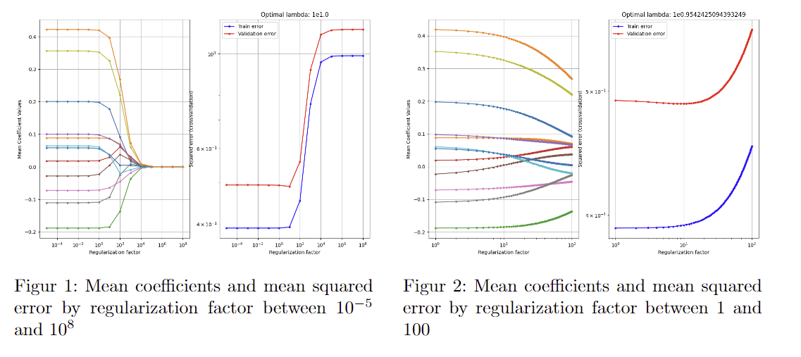
The figures show that the validation error is the lowest just around 10. We get the optimal lambda value to be 9. This is quite a strong regularization parameter, which means large coefficients are severely punished, this often means the model is less complex than an unregularized one. This strong of a lambda definitely influences the model, but isn't so large to overly constrain the model.
When we use the model with the lowest generalization error, which was found earlier, we can see the weights of each feature. They are listed below
We see the model weights our offset attribute really high, which means there is a high baseline value of alcohol. We see that the more magnesium, proanthocyanidins, malic acid, color intensity we have, the less is the alcohol percentage. The second highest weight is the Hue, which is the color of the wine. I didn't understand that was possible, since rum and gin have the approximately same alcohol percentage but two different colors, but then again this is wine, the ingredients are very much different and therefore also the colors.
In this section we will create an artificial neural network (ANN), a linear regression and a baseline model, we will train them with two-level cross-validation and compare them. We create a k-fold, where we will let K1 = K2 = 10. For each iteration of the inner loop, we test the different hyperparameters. For ANN it's the amount of hidden units, which is in the range of 1 and 5. For our linear regression model the hyperparameter is the regularization parameter which is in the range of 10-5 to 109. There is no hyperparameter for the baseline model We get the following data
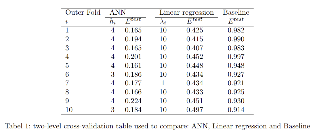
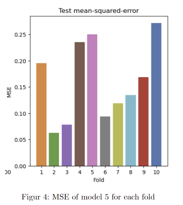
We can see that generally with the neural network the best amount of hidden units is 4, with some at 3. and the linear regression mostly λ = 10 . the best model for the neural network is model 5 with a mean squared error (MSE) equal to 0.161 and for the linear regression is model 3 with a MSE equal to 0.407.
To compare the models we use a paired t-test to see if there is a significant difference between the three models. This can be enabled since we use the same folds each time.
A series of paired t-tests were performed. Below are the summarized results:

When the p-value is under 0.05. We can conclude there is a significant difference. All the tests show a p-value under that meaning all tests are significant different. ANN generally also has a much lower MSE than the linear regression, where the average difference is 0.2573
In the following figure we can see what a neural network looks like and behaves, we got 12 inputs that go through the hidden layer and end up with one output, which is that models predictions.
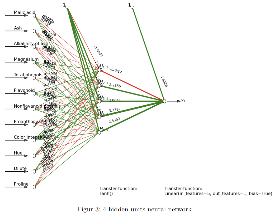
in figure 2 we can see what a neural network looks like and behaves, we got 12 inputs that goes through the hidden layer and ends up with one output which is the prediction. Overall we see that the way to estimate the alcohol is the neural network and we would definitely recommend to use it for this type of regression.
Classification
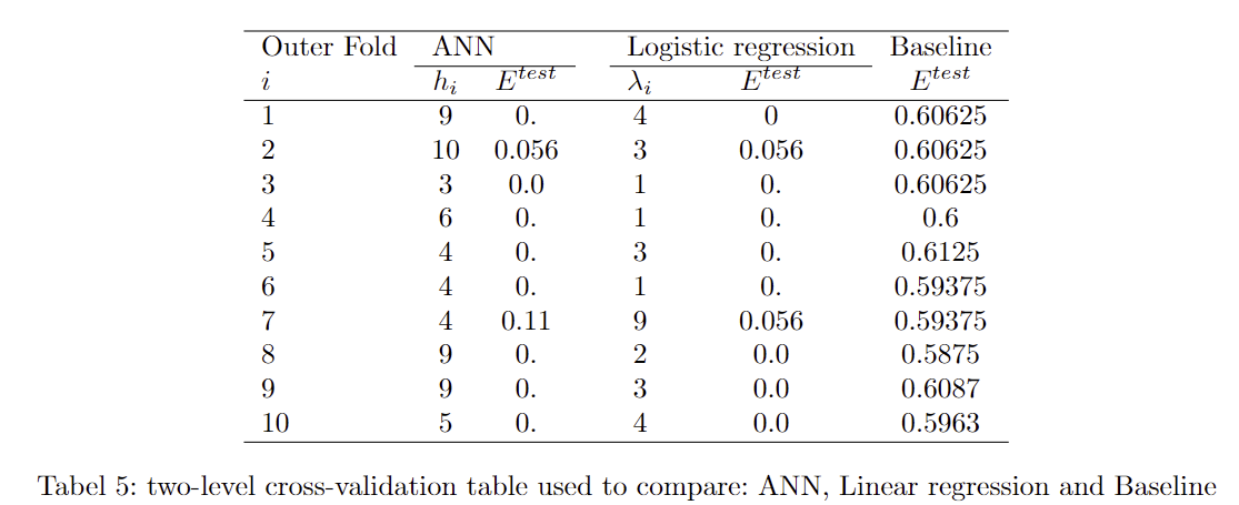
The dataset is setup for a classification with the 3 cultivators. This means we have a multiclass classification problem. We have chosen to use the ANN model for our model 2. Our three models is then a Logistic regression, an ANN model and our baseline model.
Discussion
From this project we have learned to work with different forms of regression and classification. We can conclude the neural network works better in this instance of regression, where the model had to guess the alcohol content of the wine. The logistic regression for classification worked well and in this instance made 1 error less than the ANN. When we look at the p-value, we can see there is no significant difference. So we can't conclude which is better. From working with classification we learned to use the McNemar test in a practical way and not just theoretical. On top of that, we got a lot of experience fine tuning the neural networks and adjusting data sets to fit the models. Plus Plenty of debugging experience.
Our data is used in the paper "Comparative analysis of statistical pattern recognition methods in high dimensional settings" publicized 20. December 1993.
In the paper, the authors compare different classifications methods to see what works best. we have not used any of the methods we they have used. and our classifications would rank 2. and 3. with 99.9888% for our our regression and 99.833% for the neural network. but this paper is soon 30 years old, but still holds some of the most fundamental methods such as KNN.
In conclusion the dataset is really nice to work on, when it comes to classification and regression.