In this blog we examined the interaction between frustration levels and heart rate during two-person puzzle-solving tasks. We employed statistical tests to determine assumptions and thereafter conducted further testing to find that there was no statistically significant effect of frustration on the proxy heart rate metrics, although aside from this we did find an effect of whether or not one was the solver or instructor in the given tasks. Furthermore we created several AI models on a trinarized version of the given data and found that if there are underlying patterns that could result in a classifier that would perform better than an extremely simple baseline, we could not find them. As a further exploratory task we tested the models on the individual level, and from this we found that the KNN model was the most robust, with the ANN being the least.
Introduction
This report presents an analytical study of a dataset consisting of 168 observations, each with 13 features, centered around heart rate and frustration levels during puzzle-solving tasks. Employing a range of statistical tests such as Shapiro-Wilk, ANOVA, and Kruskal-Wallis, along with AI models like Artificial Neural Networks, K-Nearest Neighbors, and Multinomial Logistic Regression, the study aims to discern patterns and relationships within the data. This analysis further aims to determine whether the potential applications of AI in interpreting complex relationships in the dataset are relevant.
Description of the data
The dataset contains 168 observations with 13 features each. The dataset is from an experiment, where the heart rate and frustration level were measured while the participants competed in solving different complex puzzles. One must note the heart rate metrics are proxy measurements since the actual heart rate isn't in this subset of the data. The 13 features are HR\_Mean, HR\_Median, HR\_std, HR\_Min, HR\_Max, HR\_AUC, Round, Phase, Individual, Puzzler, Frustrated, Cohort. There are two cohorts, each containing the data on the participants who performed these tasks. The cohorts contain 6 and 8 people respectively. Each person was given an E4 sensor and was instructed on how to use it. For the experiment, the cohorts were divided into teams of 2 and competed, where you were either the puzzle-solver or the instructor. Each experiment consisted of 4 rounds with 3 different phases, with rest and calibration spread out between them.
This means the number of observations per round per person was 3, split into pre-puzzle with frustration level, active puzzle with frustration level, and post-puzzle with frustration level. %% kan nok godt forklares bedre. The participants were from a university department and were recruited from an interdisciplinary research group with students and employees from the university. The men and women ranged between 20 and 42 years old.
Methods & analysis
The feature frustrated had potentially 11 classes ranging from 0 to 10. Since there are no observations with 9 or 10, we only have 9 classes. The lower levels of frustration has multiple observations whereas the higher ones had only a handful or fewer. For this reason we have trinarized frustration into 3 classes low (0,1,2), medium (3,4,5) and high (6,7,8).
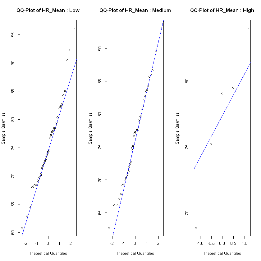
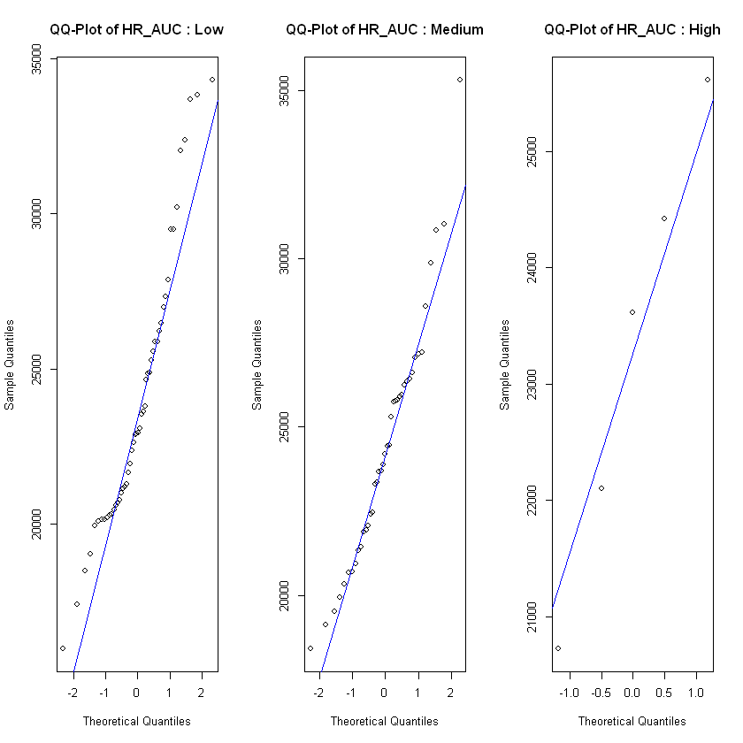
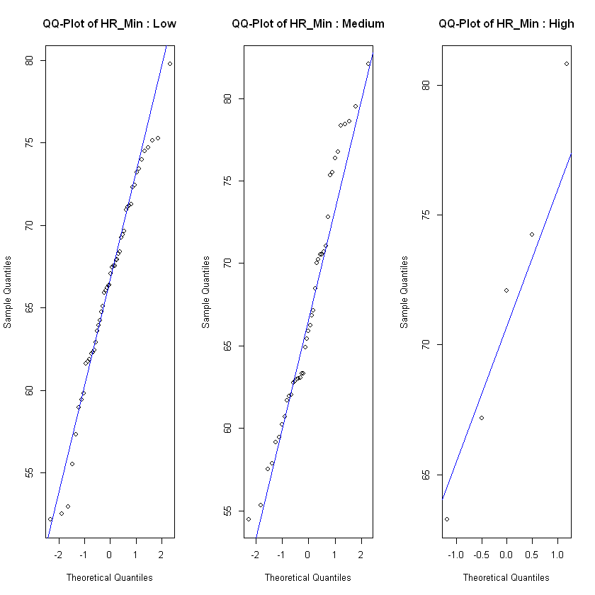
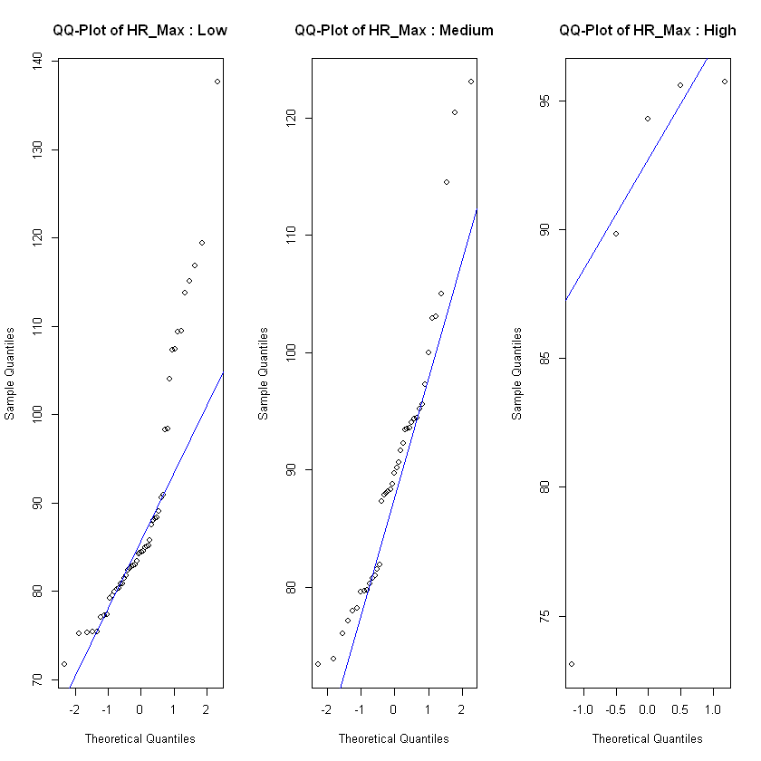
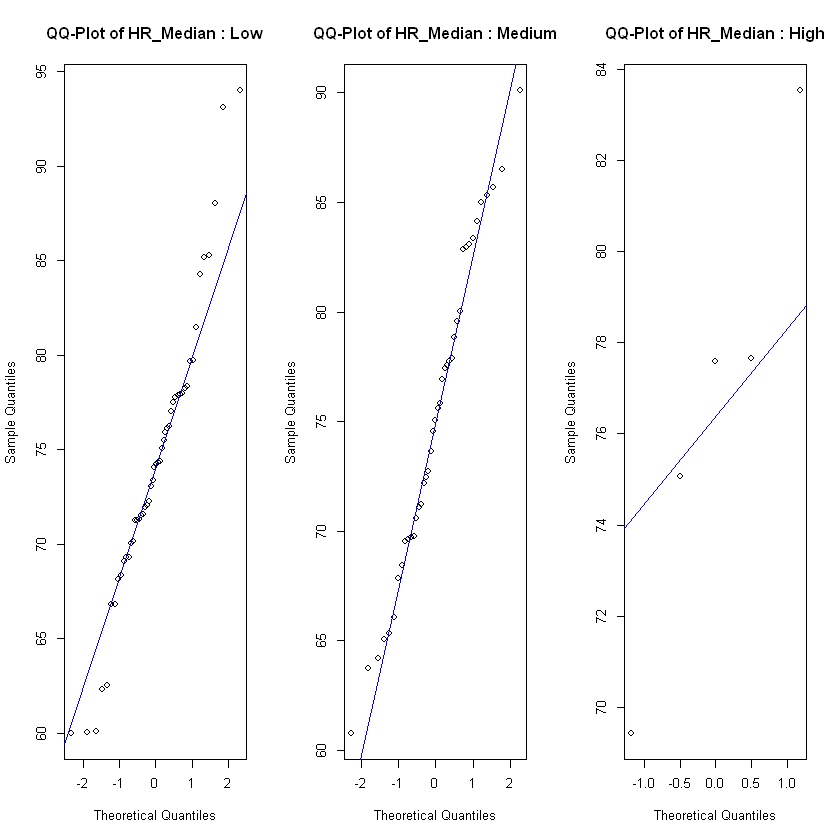
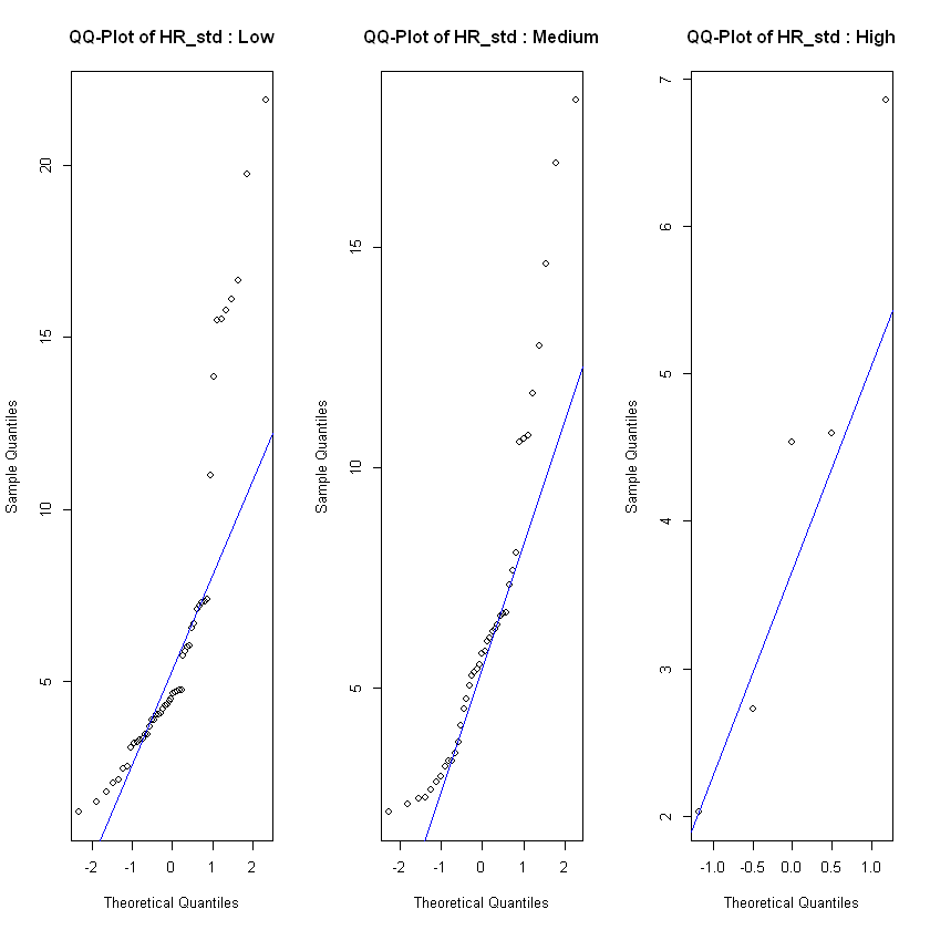
In order to see if the level of frustration impacts the heart rate, we test each of the heart rate features on the observations in each class low, medium and high for different assumptions. For normality assumption we test with a Shapiro Wilk test and also use QQ-plot. If the feature is normal distributed across all classes we test for homogeneity of variance with a Levene's test. If the feature fulfills the assumptions of normal distribution and equal variances, we test for effect with an ANOVA test. For the features that weren't normal distributed on all classes of frustration we use a Kruskal-Wallis test to test if there is a significant difference between heart rate and level of frustration. If the Kruskal-Wallis test show significant difference we use a Dunn's test to specify where the interactions are, not only if they exist or not.
In the experiment there are two roles, the puzzler and instructor. To see if they have any significance on each of the heart rate features or the frustration feature, we conduct the following tests. We use a chi squared test to determine if the puzzler role has a significant effect on the level of frustration. But for the effect on heart rate, since the data is numeric and not categorical we can use a classic t-test to determine whether or not there is a measurable effect. Afterwards we conducted post-hoc analysis just as before using Dunn's test.
Now that we have checked all the relevant assumptions of the data, and seen that there is no significant effect of frustration on any of our heart rate metrics, as they all had similar effects.
After these prerequisites have been taken into account, the next step was to use the models we have chosen to build a classifier. The models chosen are as follows:
Baseline model:
This model is a normal prerequisite for statistical evaluation that we use as a tool to determine how good our other models are relative to the simplest possible classifier. Here we simply let our classifier choose the most common class for every prediction.
Artificial Neural Network:
This model uses a neural network trained to have certain weights and biases, to predict which class the new data is. Our neural network has 5 hidden layers plus a skip-layer and a maximum number of iterations at 500. This model was chosen because the interaction between frustration and heart rate was undetectable by ANOVA or Kruskal-Wallis tests. Therefore an ANN, which by design is adept at detecting complex and obscure patterns in data, became a clear choice.
K-Nearest Neighbors algorithm:
This model looks at each point in the data set based on it's k = 31 nearest points based on numeric distance, then classifies based on a majority vote among those neighbors. This was slightly problematic given the large difference in ranges between features, therefore we scaled all the predictor features (heart rate metrics) using R's inbuilt scale() function. This model was chosen also based on our data's noisiness and complexity, KNN is a non-parametric test and therefore a very safe choice. In order to find the most optimal K we tested k=1, 2, 3, ... , 200. Multiple K values performed equally well and we took the lowest "optimal" number, which we found to be 31 for the trinarized data.
Multinomial Logistic Regression:
This model uses logistic regression to classify on multiclass data. It fits a function to predict what to classify the new data as. Because of the lack of direction given by the ANOVA and Kruskal-Wallis test we chose to include all proxy heart rate metrics in order to predict the classification of frustration.
We have chosen cross-validation, as our dataset was not big enough to just do a test-train-split. We have chosen to use a stratified k-fold, as the groups are unequally distributed, and to train the data on all the possible classes. Other than that will we test the models robustness by using group-k-fold excluding one of the cohorts to see how it handles unseen data.
In order to evaluate, which model performs best, we check if a model classifies correctly for each observation, showing 1 if correctly guessed and 0 if wrongly guessed. Once this is established for all models we can compare two models at a time by setting up a contigency table. When the contigency table is established we use McNemar's test on the tables.
Results
After checking the relevant assumptions and conducting ANOVA or Kruskal Wallis. We tested all heart rate metrics that fulfilled the assumptions of normality and homoscedasticity against the frustrated level and found that there are no significant differences between the means of the different groups, meaning the ANOVA tests suggest that there is no significant effect of frustrated on the heart rate. Then on the heart rate metrics that did not meet those assumptions, we conducted a Kruskal-Wallis test. The results from this test mirror the previous ones and show that there is no provable effect of frustration on heart
Our next step was to conduct similar analysis except analysing the "Puzzler" variable. We conducted similar assumption checking and analysis compared to the previous section. The T-tests conducted in this phase revealed that there was a significant effect of being a puzzler on multiple heart rate metrics as seen in table 1, but none on the frustration levels.
| Metric | t_statistic | p_value |
| HR_Mean | 3.5287039 | 0.0005413543 |
| HR_Median | 3.6674164 | 0.0003300847 |
| HR_std | -0.4716527 | 0.6377940814 |
| HR_Min | 2.9451863 | 0.0036930557 |
| HR_Max | 1.2433875 | 0.2154804815 |
| HR_AUC | 2.4969098 | 0.0135131656 |
From table 5 we can see each fold of the cross-validation and the average accuracy for the models. From this, it is possible to see our models have not performed perfectly and our best model aside from the baseline is our KNN with an accuracy of $\approx 62\%$. But none of our models would be better than our baseline, which just guesses the most common category, but the results may be skewed because of the huge discrepancy between the distributions of each frustration class.
| Outer Fold | ANN | KNN | MLR | Baseline | |||
| i | Acc | Acc | Acc | Acc | |||
| 1 | 0.521 | 0.521 | 0.510 | 0.521 | |||
| 2 | 0.014 | 0.597 | 0.653 | 0.764 | |||
| Average | 0.267 | 0.559 | 0.582 | 0.642 |
We then tested the robustness of the models. We separated the data in cohorts and ran a group-K-fold to see, how well our models handles not seeing the other cohort. The result in table 2, shows that the ANN, handles the unseen data worst by far, only getting $1.4\%$ when the only data it had seen was the data in cohort 2. And our baseline got even better, getting an accuracy on $64.2\%$ due to the difference in size by the cohorts. Whilst the two other models were around the same accuracy as previous mentioned in table 5. The problem with the ANN could stem from overfitting the model, it could also be because of cohort 2 having a distribution of 55 low, 12 medium and 5 high that may have had an impact on the guesses the ANN made.
On the trinarized data we tested our models and compared them to each other with contigency tables and McNemar tests, which gave the following results from table 3
| ANN vs KNN | ANN vs MLR | |||
|---|---|---|---|---|
| 0 | 1 | 0 | 1 | |
| 0 | 62 | 2 | 34 | 30 |
| 1 | 3 | 101 | 30 | 74 |
| ANN vs Baseline | KNN vs MLR | |||
| 0 | 24 | 40 | 39 | 65 |
| 1 | 31 | 72 | 24 | 41 |
| KNN vs Baseline | MLR vs Baseline | |||
| 0 | 33 | 32 | 23 | 41 |
| 1 | 39 | 64 | 40 | 64 |
As our exploratory task we chose to again test the models for robustness, we did this by performing group-k-fold on the individual, so one or more groups were left out. From this we got the result where, again the KNN outperforms the other models. While the accuracy on the unseen data, implies that the ANN model underperforms heavily in regards to robustness.
Discussion & Conclusion
In conclusion, this study, which analyzed a dataset provided to us, focused on understanding the relationship between frustration levels and heart rate during puzzle-solving tasks. Our findings have been largely inconclusive. There was no indication of interaction between any of our proxy heart rate metrics and frustration levels, regardless of test used. These results could easily be explained by the vast imbalance in our dataset, along with the extreme lack of data points in most of the higher frustration levels.
The models employed, including an Artificial Neural Network, K-Nearest Neighbors, and Multinomial Logistic Regression, demonstrated varying degrees of effectiveness, with none outperforming the baseline model. Although it is worth noting that KNN was clearly our most robust model when shown new or unseen data. The reason for our models' low performance is likely the fact that the data we received was not only an approximation of the data that we are actually interested in (heart rate) but even the data that is not an approximation (Frustrated) is a highly relative scale that varies from person to person, and we have no way to determine if a "2" on the frustration scale is equal for every tested individual. Along with this the data we have is even a subset of the entire dataset, confounding our results even more. All of this noise in the data makes it extremely hard to determine any useful way to apply an AI model or tool to this dataset. These results highlight the complexities in dealing with proxy data and suggest the need for purpose-driven and thorough data collection, cleaning, and presentation procedures, as well as the importance of diversity and extensivity of the relevant datasets.
Appendix
